
A formula for success: reviewing the social discount rate
The social discount rate (SDR) is a crucial component of the UK government’s approach to project and policy appraisal. Government guidance has stipulated the same SDR (3.5%) since 2003. In the first of two Agenda articles, we show that recent research can reasonably support an SDR of under 2.5%; and that this SDR declines considerably more slowly as the appraisal period is extended than the one that is currently used.
SDRs enable us to place a present value on the future costs and benefits of projects and policies that are intended to provide a societal benefit: they specify the degree to which we ‘discount the future’. SDRs are largely unrelated to discount rates used to appraise private projects, such as the weighted average cost of capital (WACC).
Identifying the ‘correct’ SDR is one of the most important aspects of cost−benefit analysis, as changing the discount rate by even a fraction of a percentage point can affect whether a policy is approved. In this article, we show that a case can be made for reducing the current UK SDR by over 1%.
It is often debated whether an SDR ought to reflect the rate that society should discount at (prescriptivism), or the rate that it does discount at (descriptivism). Here, we do not take a position on which is more appropriate, as this is more of a question for moral philosophers than for economists. Prescriptivist arguments for changing the SDR would state that the current SDR does not represent how society should trade off consumption across time, while descriptivist arguments might claim that empirical facts have changed or become better understood over time, and that the SDR should therefore be adjusted to reflect this.
Since 2003, the UK Treasury’s Green Book (which provides guidance on appraisal and evaluation to inform government decision-making) has stipulated an SDR of 3.5% in real terms, based on a formula that represents the socially optimal discount rate, r:1
r = δ + L + μg
Table 1 describes the four parameters and their current values, which together result in an SDR of 3.5%. The parameters are discussed in more detail below.
Table 1 Elements of the SDR
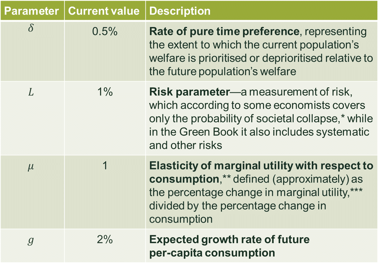
Source: HM Treasury (2018), ‘The Green Book’.
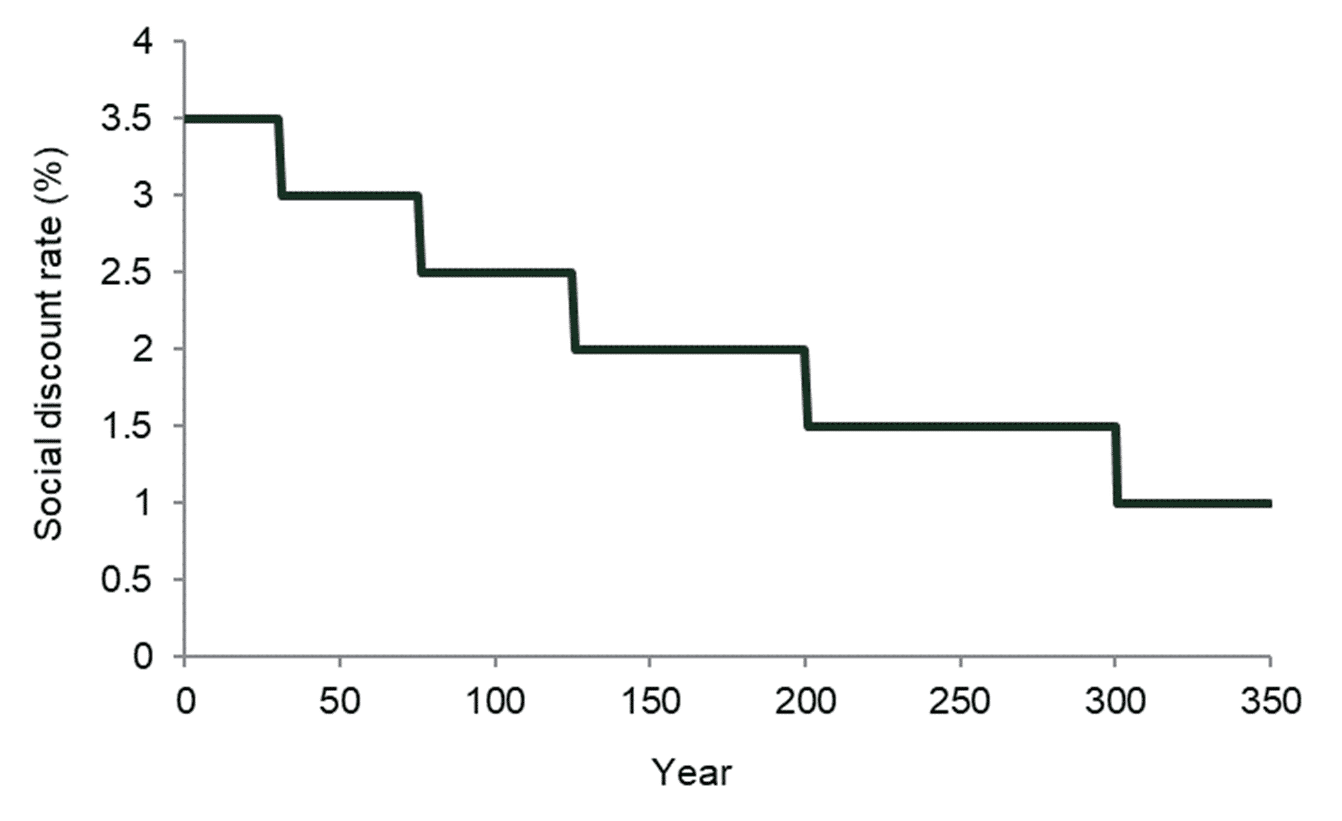
The above formula shows how the SDR is calculated for projects that are evaluated over 30 years or less. In the case of longer-term projects, a long-term SDR is calculated. This results in a formula for the SDR that differs from the equation above by making the SDR a function of time. Consequently, after 30 years, the SDR in the Green Book declines from 3.5% in accordance with the term structure shown in Figure 1. This term structure was described in a 2002 report by Oxera that summarised the research available on the subject at the time.2
Figure 1 The term structure of SDRs in the UK
The remainder of this article discusses the parameters of the SDR equation. The rate at which the SDR should decline, whether it should be adjusted for inequality, and the implications for UK policymaking, will be covered in a future Agenda article.
The rate of pure time preference
The rate of pure time preference (δ) represents the relative weight that is placed on the welfare of people alive now versus people alive in the future.3
A δ of 0 implies that equal weight should be placed on current and future people’s wellbeing, while δ > 0 implies that the current population’s welfare counts for more, and δ < 0 implies that it counts for less.
Currently, the UK government sets δ at 0.5%,4 based on the median result from a survey of experts.5 While the value δ = 0.5% may seem very close to δ = 0, the former implies that the welfare of people alive in 139 years is worth half that of people alive today. This is potentially inconsistent with many people’s moral intuitions.
While several arguments have been made for δ > 0, one of the most famous is by economist Kenneth Arrow who showed that, when δ = 0 (and under other additional assumptions), we are led to claim that current generations should save over two-thirds of their income for the benefit of future generations.6 Arrow contended that this was implausibly high, and that therefore δ should be greater than 0.
There are, however, (at least) two reasons why a δ of 0 could be reasonable.
- The assumption that δ = 0 reflects the view that the value of a person’s wellbeing does not depend on when that person is born. This view was operative in the Stern Review;7 and according to the Intergovernmental Panel on Climate Change, it is the majority view among economists.8
- Since 2003, society has become increasingly concerned for the welfare of future generations—exhibited, for example, by the current focus on climate change and plastic pollution. In Wales, the government even passed a ‘Well-being of Future Generations Act’, requiring the government to consider long-term impacts in policymaking.9
Therefore, even if δ should not be reduced all the way to 0, it could perhaps be brought closer to this value. It should also be noted that the results of the expert survey referred to above may be consistent with a belief that δ = 0, because the survey did not separately identify δ and L, meaning that experts’ estimates may have covered δ + L rather than δ alone.
Does the current model treat risk correctly?
The risk parameter L (measured at 1% in the Green Book) captures unforeseeable factors that could significantly reduce or completely eliminate the benefits associated with a project.10 It also includes a small premium for ‘systematic’ risk, to account for the fact that the net benefits of a project are typically positively correlated with real GDP growth.11
Consequently, L captures a mixture of different types of risk, instead of considering each of them in different ways. This is described by Freeman, Groom and Spackman (2018) as a ‘practical shortcut’ for taking risk into account.12
In reality, projects face three types of risk that can affect their net benefits:13
- project-specific risk (unsystematic risk)—for example, the probability that a project will be managed well or badly, leading to over- or underperformance;
- factors outside the project’s control (systematic risk)—for example, the risk that the level of benefit it provides will be correlated with changes in the macroeconomic environment, such as economic growth. This risk cannot be eliminated through diversification (i.e. having lots of different projects);
- catastrophic risk, reflecting the probability that society will ‘fail to survive’ a given year. Catastrophic risks come from existential threats such as meteorites as well as significant political events such as large-scale anarchy or nuclear war.
With each of the above, an increase in risk should intuitively raise the SDR because the future benefits of a project are more likely to be reduced, or—in the event of catastrophic risk—destroyed, making future investment less attractive.
While there does not appear to be consensus on how the different types of risk should be treated, we outline below an approach that could be taken.
Unsystematic risk could be dealt with through explicit adjustments to the profile of benefits and costs, as is already suggested in the Green Book. Methods for doing this include decision trees and real options techniques, which directly adjust the streams of benefits and costs rather than the discount rate.
Systematic risk can be dealt with in two ways: analysts can either convert net benefits into certainty equivalents14 and then discount them at an SDR where L represents only catastrophic risk (sometimes called a ‘risk-free’ SDR), or they can keep net benefits as they are and add a term for systematic risk to the SDR.15 In the context of policy appraisal, economists differ in opinion on the importance of systematic risk, based mainly on whether they take a normative or a descriptivist approach to discounting. In the former case, systematic risk is often quantified at below 0.1%,16 while in the latter case it is considerably larger, with one estimate putting it at 2%.17 Some economists who take the former approach consider that systematic risk can be largely ignored for government projects.18 The question of which is the correct treatment is clearly material, but also highly complex and controversial.
Catastrophic risk could be captured by a parameter reflecting the probability of societal collapse. As this risk is independent of other macroeconomic events (unlike systematic risk), it would enter L directly and linearly. This would essentially result in L being set to equal catastrophic risk, as in the Stern Review,19 in which catastrophic risk was estimated at 0.1%, implying a probability of society’s survival after 100 years of approximately 90%.20 Toby Ord, a philosopher at Oxford University’s Future of Humanity Institute, places the probability of the complete destruction of humanity at approximately 17% across the next century, implying an estimate for L of around 0.2%.21
If systematic and non-systematic risk are removed from L then its role in discounting will change to focus exclusively on catastrophic risk.
The elasticity of marginal utility
The elasticity of marginal utility with respect to consumption (μ) reflects three conceptually distinct features of a social welfare function:
- the level of intratemporal inequality aversion—the aversion that a society has to (consumption) inequality at a given point in time;22
- the level of intertemporal inequality aversion—the aversion that a society has to (consumption) inequality across time;
- the level of risk aversion—the extent to which a society is concerned about not just the central estimate of a project’s net benefits, but also its variance.
As mentioned above, μ measures the percentage change in marginal utility (i.e. the rate at which an individual’s wellbeing changes as their consumption increases) caused by a 1% increase in their consumption. Higher levels of μ reflect a society that derives less utility from higher levels of consumption than would be the case if μ were lower.23 Such a society therefore benefits less from shifting resources to the future (assuming that the society is expected to become wealthier in the future). Two issues arise with the estimation of μ.
First, some economists take the view that the elasticity of marginal utility depends on how society should value consumption, whereas empirical analysis uses real-world data and so is based on the actual behaviour of individuals. Disagreement on whether μ should be empirically estimated can have material implications for its magnitude, because normative and empirical economists will use different methodologies. For example, empirical economists will be happier using real-world data, while normative economists may test the implications of different values of μ for various ethical thought experiments. Empirical methods were used to derive the value of μ = 1 used in the Green Book, while some academics who prefer normative methods have found higher values, such as between 1.5 and 3.24
Second, to the extent that empirical methods are appropriate, there is debate over which methods should be used and the values that they suggest. Empirical estimation is particularly difficult in the case of μ because, as discussed above, it measures three conceptually distinct aspects of social welfare functions, and methods based on one of the three aspects may not produce results that are consistent with methods based on another.
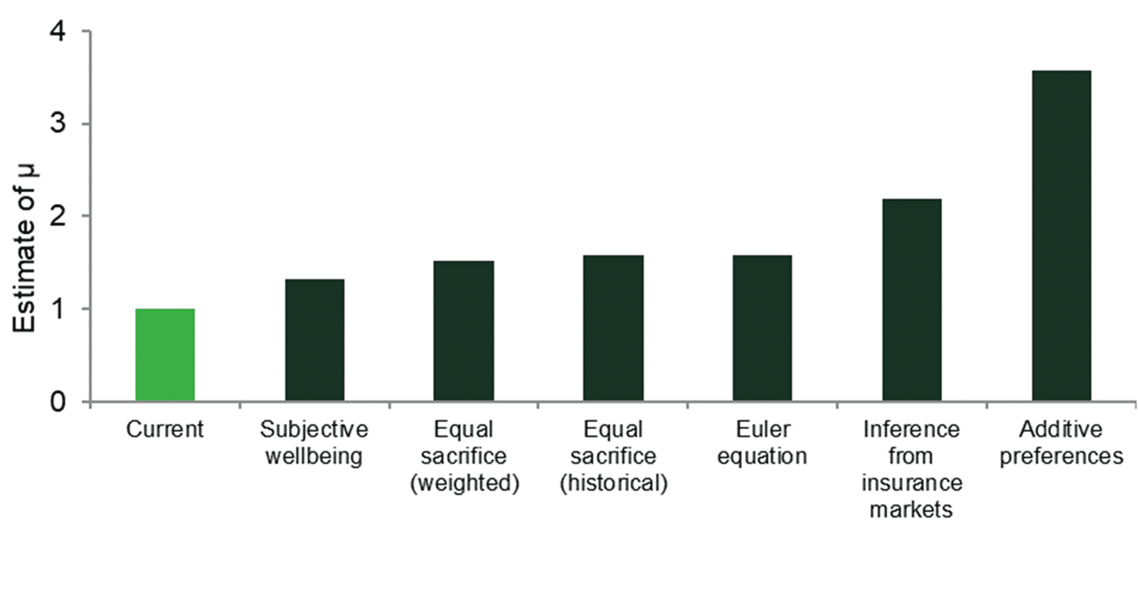
Notwithstanding this, the Green Book currently sets a value of μ = 1, based on results presented in Oxera (2002), which drew on available research at the time to suggest a value of between 0.5 and 1.2.25 Since 2002, more work has been done on the estimation of μ—most recently in Groom and Maddison (2019), whose ‘central’ estimate was 1.5.26 While any values will be dependent on the particular estimation method adopted, and the estimation method may or may not be disputed, Figure 2 shows that all of the μ estimates are higher than 1 (the current value), indicating that an increase may be appropriate.
Figure 2 Comparison of current value of μ with empirical estimates by Groom and Maddison (2019)
The growth rate of consumption
The growth rate of consumption, g, attempts to capture the expected percentage change in real per-capita consumption. This is currently 2% in the Green Book. Higher rates of expected consumption growth increase the SDR because they imply that future generations will be wealthier, meaning that the benefit of providing them with additional consumption will be lower.
The 2% estimate is based on a 1.9% long-term real GDP growth forecast from the UK Office for Budget Responsibility (OBR), and historical estimates of consumption growth, which are typically also close to 2%. However, there are two reasons why this estimate may need to be revised downwards.
First, the precise estimate for g is highly dependent on the time period that is analysed. This is shown in Figure 3, which plots the average growth rate for the 20 years prior to the year on the x-axis, and demonstrates that these have declined since around the 1981−2001 period and are now closer to 1.5%. This is consistent with the latest Fiscal Sustainability report from the OBR, which expects consumer spending to increase by 1.4−1.5% per year once the economy recovers from the COVID-19 pandemic.27
Figure 3 20-year average growth rates
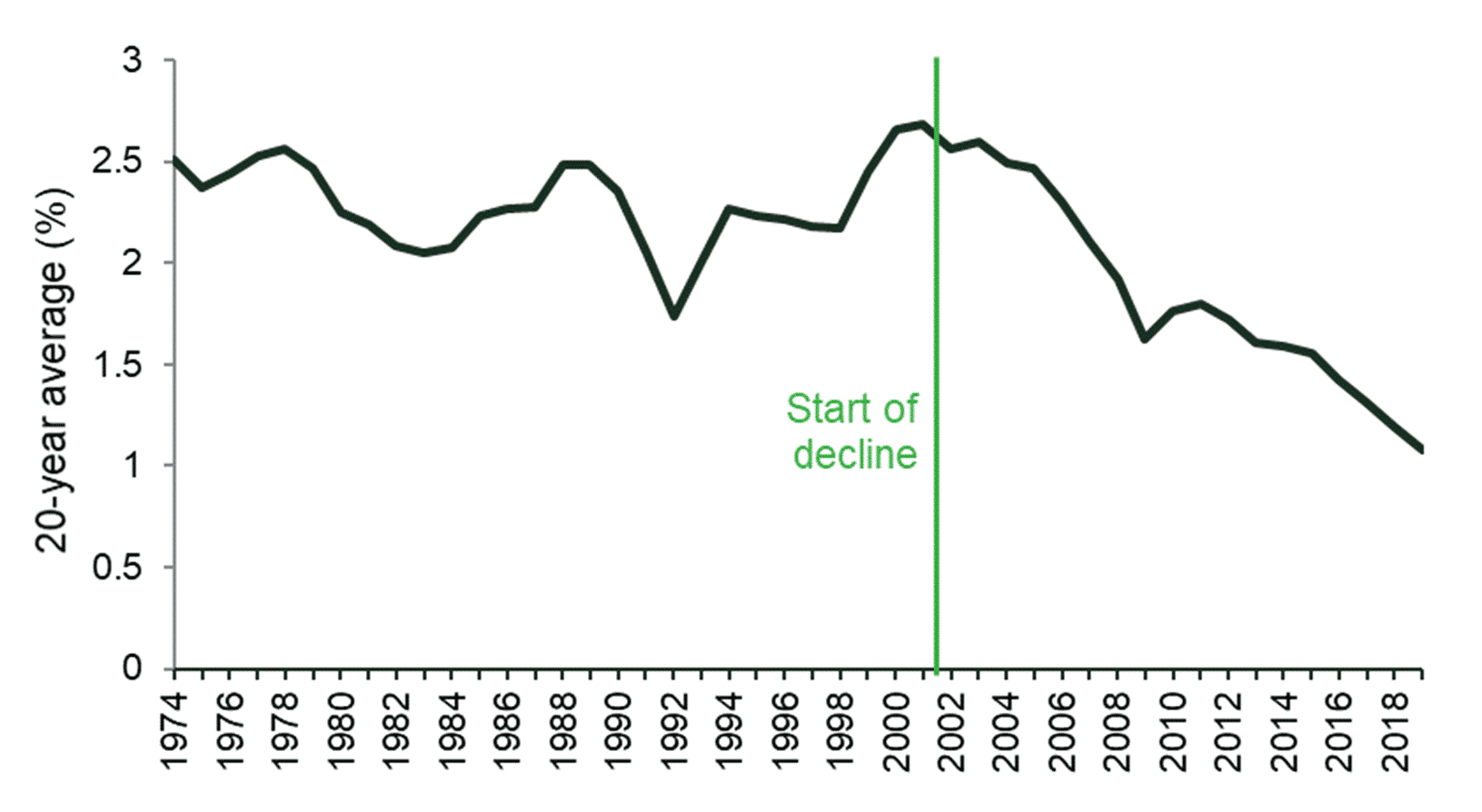
Source: Office for National Statistics.
Second, an optimal estimate of g should cover the consumption of both economic goods and services (i.e. those that are measured by the GDP and consumption statistics mentioned above) and non-economic goods and services (such as biodiversity, which is not measured in official statistics). If consumption of economic goods tends to reduce that of non-economic goods—for example, because the former causes pollution, which reduces biodiversity—then estimates of g based on GDP or consumption data alone would be overestimates, because they would ignore the fact that consumption of non-economic goods was decreasing. This would result in an overstated SDR.
Two possible approaches
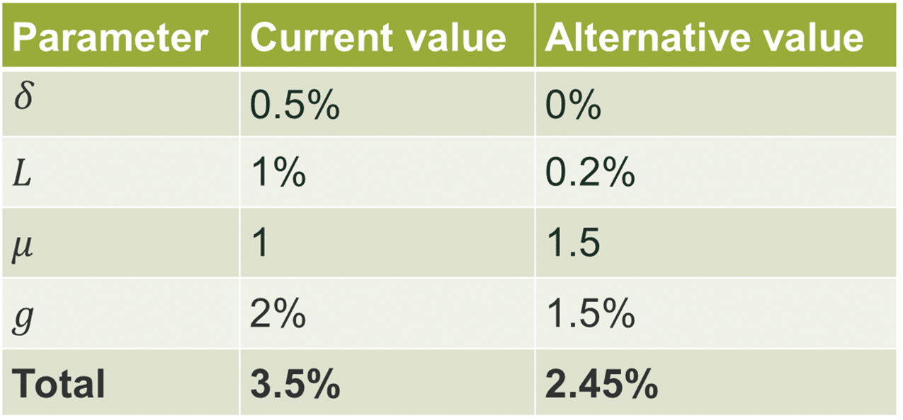
Recent research suggests that many of the parameters in the SDR could be changed. In all cases except for μ and L, the indication is that they should be reduced. Table 2 shows that the net effect of defensible changes would be to reduce the SDR from 3.5% to 2.45%.
Table 2 Comparison of current and alternative SDR parameterisations
Source: Oxera.
The reduction from 3.5% to 2.45% is not necessarily a change that should be made, but the material difference between the current approach and this alternative suggests that consideration ought to be given to whether the current approach is still appropriate in light of the latest evidence.
With the exception of L, the changes in Table 2 all represent updated estimates of parameters whose conceptual role has stayed the same. In the case of L, however, the parameterisation reflects the normative approach to systematic risk, where it is considered to be relatively immaterial (in the public policy context). If the descriptivist approach were taken, the SDR would be considerably higher. The adoption of the normative approach should not be read as an endorsement, but merely as one defensible approach that is selected for illustrative purposes.
The second article in this series will cover further potential changes to the SDR. In combination with the above discussion, we will then present a consolidated picture.
1 The formula is derived from a model that assumes no externalities, identical individuals (i.e. no inequality), and no uncertainty.
2 Oxera (2002), ‘A social time preference rate for use in long-term discounting’, 17 December.
3 This is not the same as the relative weight of current and future generations’ consumption, which is determined by the SDR as a whole. This means that the rate of pure time preference is conceptually distinct from the risk-free rate used in private project appraisal, often implemented through mechanisms such as the capital asset pricing model (CAPM), which weights intertemporal consumption.
4 For long-term interventions, however, analysts performing cost−benefit analyses of policy have to present their results with both δ = 0 and δ = 0.5%.
5 The Green Book refers to a 2018 paper by Freeman, Groom and Spackman, which in turn refers to a 2015 paper by Drupp, Freeman, Groom and Nesje. See HM Treasury (2018), ‘The Green Book’, p. 102; Freeman, M., Groom, B. and Spackman, M. (2018), ‘Social Discount Rates for Cost−Benefit Analysis: A Report for HM Treasury’, p. 8; Drupp, M. A., Freeman, M. C., Groom, B., and Nesje, F. (2015), ‘Discounting disentangled’, American Economic Journal: Economic Policy, 10:4, pp. 109−34.
6 Arrow, K. J. (1996), ‘Discounting, morality, and gaming’, presented at the EMF−RFF Conference on Discounting, 24 December.
7 Stern, N. (2007), ‘The Economics of Climate Change: The Stern Review’, 30 October.
8 Intergovernmental Panel on Climate Change (2014), ‘Social, Economic, and Ethical Concepts and Methods’, p. 229.
9 Future Generations Commissioner for Wales, ‘Well-being of Future Generations (Wales) Act 2015’.
10 More precisely, it measures only those risks that are not explicitly modelled as streams of costs or benefits.
11 HM Treasury (2018), ‘The Green Book’, p. 102.
12 Freeman, M., Groom, B., and Spackman, M. (2018), ‘Social Discount Rates for Cost−Benefit Analysis: A Report for HM Treasury’.
13 See, for example, the discussion of how to appropriately adjust for different types of risk on p. 4 of Freeman, M., Groom, B. and Spackman, M. (2018), ‘Social Discount Rates for Cost−Benefit Analysis: A Report for HM Treasury’.
14 A certainty equivalent is defined as the guaranteed amount of money that an individual would view as equally valuable to an uncertain amount. Projects that provide different levels of net benefit in high- and low-GDP states of the world create uncertainty, and policymakers generally prefer a project that provides lower net benefits on average, but which removes the uncertainty. The net benefit of a project with no uncertainty, that a policymaker is indifferent to relative to a project with uncertainty, is the certainty equivalent of the risky project.
15 Moore, M. A., Boardman, A. A., and Vining, A. R. (2017), ‘Risk in Public Sector Project Appraisal: It Mostly Does Not Matter!’, Public Works Management & Policy, 22:4, pp. 301−21.
16 Kocherlakota (1996) estimates that this term would equal 0.076%, while Freeman, Groom and Spackman (2018) estimate that it would equal 0.075%. Kocherlakota, N. R. (1996), ‘The Equity Premium: It’s Still a Puzzle’, Journal of Economic Literature, 34:1, pp. 42−71; Freeman, M., Groom, B. and Spackman, M. (2018), ‘Social Discount Rates for Cost−Benefit Analysis: A Report for HM Treasury’.
17 This is the estimate used in France. For example, see Freeman, M., Groom, B., and Spackman, M. (2018), ‘Social Discount Rates for Cost−Benefit Analysis: A Report for HM Treasury’, p. 12.
18 Moore, M. A., Boardman, A. A. and Vining, A. R. (2017), ‘Risk in Public Sector Project Appraisal: It Mostly Does Not Matter!’, Public Works Management & Policy, 22:4, pp. 301−21.
19 Greaves, H. (2017), ‘Discounting for public policy: A survey’, Economics & Philosophy, 33:3, pp. 391−439.
20 Stern, N. (2007), ‘The Economics of Climate Change: The Stern Review’, 30 October, p. 47.
21 This estimate covers only the probability of complete extinction, whereas for an accurate value of L, the probability of other societal collapses should also be included.
22 For precision, we reference consumption rather than income inequality because social welfare functions typically evaluate the welfare of a society based on consumption rather than income levels.
23 Greaves, H. (2017), ‘Discounting for public policy: A survey’, Economics & Philosophy, 33:3, pp. 391−439.
24 Dasgupta, P. (2008), ‘Discounting Climate Change’, Journal of Risk and Uncertainty, 37, p. 23.
25 Oxera (2002), ‘A social time preference rate for use in long-term discounting’, 17 December.
26 Groom, B. and Maddison, D. (2019), ‘New estimates of the elasticity of marginal utility for the UK’, Environmental and Resource Economics, 72, pp. 1155–82.
27 Office for Budget Responsibility (2020), ‘Fiscal Sustainability Report’, July, Table 2.2, row ‘Household consumption’ (for the years 2023 and 2024).
Download

Related

Adding value with a portfolio approach to funding reduction
Budgets for capital projects are coming under pressure as funding is not being maintained in real price terms. The response from portfolio managers has been to cancel or postpone future projects or slow the pace of ongoing projects. If this is undertaken on an individual project level, it could lead… Read More

Consumer Duty board reports: are firms prepared for the July 2024 deadline?
The UK Financial Conduct Authority’s (FCA) Consumer Duty, a new outcomes-based regulation for financial services firms, has now been in force for over six months. July 2024 will see the deadline for the first annual Consumer Duty board reports. We share our reflections on the importance of these documents and… Read More